Merging multiple time-series in InfluxDB using Flux may seem like a daunting task. This in-depth Flux tutorial will explain how to pivot, time shift and join time series in InfluxDB.
In this InfluxDB tutorial, we will show you how to create an accurate overview of multiple time series with industrial data captured in consecutive production steps. Doing this requires a proper join mechanism for combining the time series into one after aligning them with respect to time.
This tutorial is based on a real-world case we solved at Factry.io with InfluxDB in an industrial setting.
Every second of the day, production sites all around the world are generating inconceivable amounts of process data. This data is directly acquired from production lines on-site and captured in the form of process parameters. Being able to reliably keep track of these process parameters throughout the production process is essential to continuously improving manufacturing operations.
Industrial process parameters are represented as concurrent time series. They do not necessarily provide data points at a similar pace, nor are they always aligned over time. Obtaining a trustworthy overview of captured process parameters during consecutive production steps can be daunting.
Time-Series Data Explained
In brief, time-series data represents a number of different data points indexed by time. As time is a constituent of anything that is observable in our world, time-series data is everywhere. When narrowed down to a production environment, captured process parameters are distributed in time in order to become distinguishable from the process data preceding or following it.
What is the difference between time-series and relational data? In contrast to time-series data, relational data holds records that are generally referenced by an artificial identifier. These identifiers can interrelate, which crafts the relational aspect.
Pivot and Join Time-Series Data in Flux
Before you get started
On a production line, be aware that a product batch cannot be in two different production steps at the same point in time. As a result, time series measured in different production steps are naturally unaligned. Hence, before properly joining these time series into one, many of them will need to be shifted over time to get the overview right.
Furthermore, retrieving data stored in a time-series database is commonly done by using the dedicated query language Flux.
Two points about this:
- In Flux, a join can only make use of an inner join mechanism to melt multiple time series into one. As an inner join solely retains the data points for shared timestamps in multiple time series, data loss is unavoidable when dealing with unaligned time series or time series captured at different rates.
- In most use cases, only time series extracted from sensors at different production steps need to be joined. This is due to the ability to differentiate between multiple tables within one time series.
Hence, reading in sensor data generated by multiple sensors at the same production step, table by table, allows us to bundle the sensor data. By ‘pivoting’ the tables into one, a time series is forged. Prior to being joined with the sensor data captured from another production step, the time series is shifted to align with respect to time. However, note that this requires all sensor data (potentially from different sensors) from one production step to be aggregated in the same way, omitting any differences in the rate at which it has been captured.
Use Case: Welcome to the Cardboard Factory

There are some best practices for pivoting and joining time series data in Flux from consecutive production steps. In this example, sensor data is captured from a replicated production site that is manufacturing cardboard panels out of recycled paperboard rolls.
The production process of the cardboard factory consists of three different steps, which we’ll refer to as entries A, B and C.
- In entry A, production starts with recycled paperboard rolls; the width and diameter of which is being measured by two separate sensors.
- In entry B, the recycled paperboard rollsare cut into paperboard sheets and processed into cardboard using a certain temperature and pressure.
- In entry C, the cardboard is cut into shape. For this entry, the height and the thickness of the panels are the key elements to be measured in terms of sensor data.
With respect to time, it takes approximately one minute for the first sheet of recycled paperboard roll to reach entry B. Further, about two minutes elapse before the paperboard sheet is processed and shaped into a cardboard panel.
Note that, in this production site, it is assumed that the speed of the production line is more or less fixed over time, making it possible to shift time series captured in different entries in order to get them aligned.
Merging Multiple Time Series Into One Using Flux
The goal in this use case is to create one trustworthy overview of all sensor data captured in each entry. Imagine today is May 4 at around 3:10 p.m. The overview should be reflecting all sensor data from the past ten minutes of the production site.
Fortunately, we are aware that the sensor data between each entry is unaligned by a few minutes. Therefore, we should be fetching data between 3:00 and 3:10 with respect to the last entry (entry C); thereby trying to align these time series with the ones from both entry A and entry B.
Think about it as being teleported to 3:10 on May 4. At that time, for a recycled paperboard roll in entry A or for a paperboard sheet in entry B, we do not yet have the sensor data for entry C. This is obviously because this sensor data will be captured only a few minutes later on the line.
With this cleared up, a recycled paperboard roll delivered by one of the suppliers is referred to in the use case as a material lot. In contrast, a paperboard sheet derived from the recycled paperboard roll resulting in a cardboard panel is mentioned as a material sublot.
At the end of the production line, a pile of cardboard panels is manufactured out of one material lot. To sum it up: In this use case, a material sublot can never be in two different entries at the same point in time, which means we need to align time series over consecutive entries.
1. Reading in the Sensor Data
First, we start by reading in the sensor data of both the width sensor and the diameter sensor for entry A. By reading in sensor data of both sensors in the same ‘filter’ (image: code snippet), we reduce this data to one time series for entry A.
In this way, we hold different tables per sensor in one time series arranged by the group key consisting of ‘_field’ and ‘_measurement’. By reducing all sensor data from one entry to one time series holding multiple tables, the opportunity arises to pivot the tables into one unified table later on.
Fetching the corresponding sensor data from entry A with respect to entry C is fulfilled by using a ‘range’ with sensor data that was captured between 2:57 and 3:07. This is applied by shifting the time range of entry A three minutes backward using ‘SHIFT_A’. Hence, for a cardboard panel at entry C, the corresponding sensor data at entry A was captured three minutes earlier.
In essence, we are mapping the time range between 2:57 and 3:07 of entry A onto the time range between 3:00 and 3:10 of entry C and, thus, onto the overview.
Note that for operations between a timestamp and a duration in ‘FROM_A’, you need to convert both the timestamp and the duration to an unsigned int to get Unix timestamps in ns prior to performing the calculation.
Entry A sensor data – code snippet
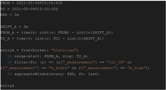
Entry A sensor data
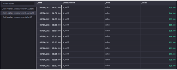
Regular and Irregular Time Series
In most use cases, the sensor data will generate a regular time series (metrics), as the time period between captured data points will be fixed. However, when working with irregular time series (events) or time series generated at a different rate, these need to be transformed into a regular time series with an ‘aggregateWindow’ to eventually build up a nice overview.
In this use case, there is only a regular time series. Therefore, retaining the ‘last’ data point for each time window of one minute should do the trick. In the case of an irregular time series, taking a ‘mean’ over a fixed time window would be the better choice.
2. Pivoting the Time-Series Data
After the sensor data from both sensors of entry A is collected into one time series with multiple tables, we now need to pivot the tables to become one. Therefore, the group key of each table needs to hold the same schema.
In this use case, the group keys schema for all tables in the time series is as follows: ‘[‘_field’, ‘_measurement’]’. To make sure that the group keys schema is identical for all tables, we can use a ‘keep’ in front of the pivot to eliminate fields that are not present in all tables.
Possible Deal-Breakers
Bear in mind that the constraint for holding an identical schema for each table in the time series can be a deal-breaker for using the pivot. Another constraint lies in the lack of being able to pivot more than one value field, although when reading in sensor data from InfluxDB, there is typically only one value field.
However, after adding some processing to the time series in Flux, chances are that an additional processed value column is present, eliminating the ability to use a pivot once more.
When performing a pivot on multiple tables in the time series of entry A, for the table rows holding a shared timestamp (row key: ‘_time’), the data point in the value field (value column: ‘_value’) will be ingested into a column determined by the name of the measurement (column key: ‘_measurement’).
In the use case, this means that the tables with the measurements ‘lot_ID’, ‘A_width’ and ‘A_diam’ will get their data points from the ‘_value’ field ingested into a separate column in the unified table, determined by their measurement names.
In terms of performance, a pivot can suffer from having too many tables in the time series to be pivoted, which corresponds to the number of active sensors in one entry. Next to that, an extensive group key schema in the pivot will also take its toll. Having a considerable amount of rows per table in the time series of an entry with ns precision timestamps can easily blow up the pivot, as well.
Finally, a small footnote on the functionality of the pivot in Flux. Keep in mind that the fields and tags that are not included in the pivot will not be ingested into the unified table. Additionally, the term pivot appears deceiving when being compared to its functionality in a relational database.
Entry A pivot – code snippet
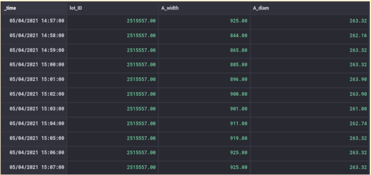
Entry A shift

3. Time Shifting the Time Series Data
Entry A
After pivoting the sensor data of entry A into one unified table, the entry A sensor data with time range between 2:57 and 3:07 gets aligned with the time range of the overview between 15:00 and 15:10 by performing a time shift of three minutes forward on the _time column.
To preserve the original timestamps of entry A, we take a duplicate of the _time column in the unified table and refer to it as the time for which a sublot actually started at entry A, mentioned as entry_A.
entry A shifted – code snippet

Entry A Shift – Code Snippet

Entry A Shift
Entry B & C
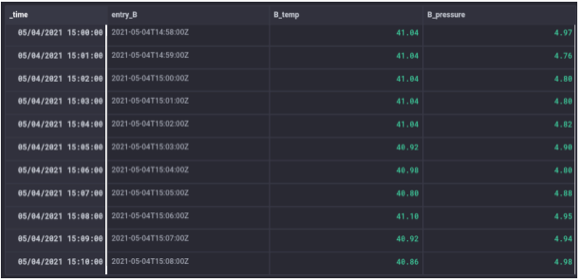
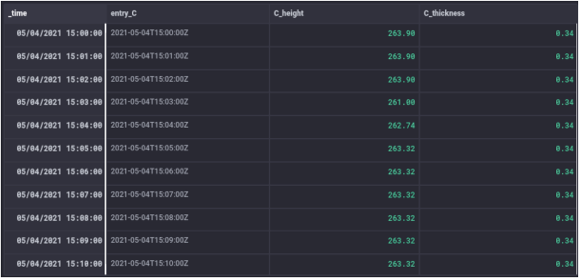
The same procedure for reading in the sensor data of entry A applies for entry B and entry C. While the sensor data for the former is shifted by two minutes to get its time range between 2:58 and 3:08 aligned with the time range of the overview, the sensor data of the latter is already in sync for the overview.
Entry B – code snippet
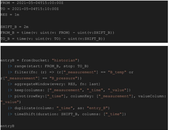
Entry B
Entry C – code snippet

Entry C
4a. Joining the Time Series
After pivoting the sensor data for each entry, three distinct time series are held, each containing one table with a separate schema and multiple value columns; for example, ‘C_height’ and ‘C_thickness’ for entry C. To create one overview, these three time series must be joined together, visualizing the data points of different sensors side-by-side with respect to time. Since the sensor data of the different entries has been formerly aligned by reading in the corresponding time ranges for each entry followed by a ‘timeshift’, the three time series can now be joined on the synced ‘_time’ column present in each of them.
Possible Issues
Since the schema differs between the three time series tables, you would encounter significant overhead when trying to pivot these three tables into one after appending them to a single new time series. Besides the superfluous complexity added, the tables of all time series are each holding more than one value column, which makes the pivot unusable in this case.
A plausible solution would be to use a ‘join’ provided by Flux on the aligned ‘_time’ column. As discussed in the pivot and join section, the ‘join’ is represented as an inner join mechanism, solely retaining data points for shared timestamps between joined tables.
In this use case, the inner join mechanism would not trigger any data loss, since only regular and aligned time series are present after the pivot. However in case of irregular time series (not using ‘aggregateWindow’ on events), time series captured at a different rate or regular yet unaligned time series, data points would get lost in the inner join mechanism.
Next to that, the ‘join’ in Flux is only letting two time series be joined together at once, which constrains the possibilities. Moreover, seen from a performance perspective, the ‘join’ is considerably less optimized compared to dedicated functions in Flux, like the ‘aggregateWindow’.
4b. Solution: Outer Join
To tackle the issues subject to the ‘join’ provided by Flux, an outer join mechanism is proposed, retaining data points for both shared and unshared timestamps between tables of multiple joined time series with respect to time. After appending the three time series to a single new time series holding one table, the outer join mechanism groups all data points by time into ‘timetables’ prior to filling up rows with the appropriate data points. Furthermore, the single complete row per timetable is extracted, preceding the ungrouping of timetables to one overview table.
Union
Once the aligned sensor data is available into a dedicated time series per entry consisting of one table, the three time series are appended by a ‘union’ to a single new time series holding one table. The ‘union’ is ingesting the sensor data of each entry vertically (image: union), meaning the table rows per entry are placed underneath each other while the resulting table schema is the union of the separate table schemas of the three time series. In this manner, you can witness ‘data point blocks’ in the resulting table referring to sensor data of each entry in the production site. Note that the ‘union’ allows more than two time series to be appended to a new single time series at once.
union – code snippet

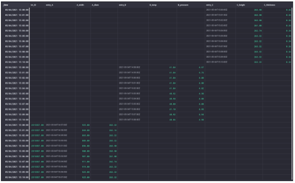
union
Timetables
The sensor data of all three entries in the single time series table is grouped by the ‘_time’ column to group the sensor data of different entries together in timetables. The ‘timetables’ refer to the tables that arise by using the group key ‘_time’ (image timetables). The forthcoming sort is fundamental to order the rows of a certain entry at the bottom of a timetable prior to starting to fill data points. In this use case the row originating from entry C is positioned at the bottom of each timetable’ by sorting for the ‘entry_C’ column in ascending order. In fact, regardless of sorting the ‘entry_C’ column in ascending or descending order, the empty data points in the ‘entry_C’ column of the rows originating from entry A or entry B will always be on top in Flux since they hold a null value.
Timetables – code snippet

Timetables
Fill
Moving forward, the data points of the columns originating from entry A and entry B are copied into subsequent rows using the ‘fill’ with ‘usePrevious’ set to ‘true’. Since the data points are filled through the bottom, the mutual order of the rows originating from entry A and entry B is not important. Note that at the bottom of each timetable, the row originating from entry C is now a complete row holding all data points for all three entries (image: fill).
fill – code snippet

fill

Extract
Finally, only the complete row at the bottom of each timetable is extracted by using the ‘tail’ with ‘n’ set to ‘1’. The timetables are ungrouped to one joined table by using the ‘group’ without any parameters to empty the group key. Check out the joined table (image: extract) and you’ll see that all sensor data originating from the three entries of the production site is visualized into one trustworthy overview with respect to the time behavior induced by a sublot passing through the production entries on site.
Extract – code snippet

Extract

4c. Outer Join Mechanism for Unaligned Sensor Data
To illustrate the outer join mechanism, one can join unaligned sensor data for the corresponding time ranges from the 3 entries in the production site into one overview. This can be arranged by removing both the ‘timeShift’ of three minutes for entry A and the ‘timeShift’ of two minutes for entry B when compared to entry C.
In that case, the sensor data of entry A will retain its time range between 2:57 and 3:07, while entry B will have a time range between 2:58 and 3:08, followed by a time range between 3:00 and 3:10 for entry C. The result is a broader overall time range for the overview than requested (image: outer join on unshifted sensor data). Besides, only unaligned sensor data is present for all three entries in the time range between 3:00 and 3:07.
Note that for the top and the bottom rows, the unavailable sensor data for a certain entry is replaced by the ingestion of null values as data points in the columns are originating from the corresponding entry. As mentioned earlier, the same principles apply for an outer join when dealing with irregular time series or time series captured at a different rate. Ideally, such an outer join mechanism should be the default behavior in Flux when performing a ‘join’.

Outer join on unshifted sensor data
Conclusion
When creating a trustworthy overview of captured sensor data at a production site in consecutive production steps, take these four elements into account:
- The step in the production process where the sensor data is captured is key to understanding the time behavior of a product batch going through the different production steps on site.
- How sensor data is captured in production indicates the urgency of using a specific time window and which selection/aggregation of data points you should obtain. Hence, sensor data can generate a regular or irregular time series or can be captured at a different rate.
- Sensor data per production step is pivoted to a time series holding one unified table of sensor data for that production step. The pivot stands out in unifying the sensor data per production step, since the different tables each referencing a sensor in that production step typically hold an identical schema when reading them in.
- Next to that, generally speaking, there will only be one data stream per sensor and thus only one value field per table in the time series derived from a production step.
- Performing an outer join on the multiple time series originating from multiple production steps, gives you the ability to create a trustworthy overview in the end. To make the most out of it, make sure to align the time series first before joining them.


